自动问答(QA)系统是一个旨在回答自然语言提出的问题的系统,根据问题的来源,我们可以简单将 QA 分为两大类:
- 1. 开放领域的自动问答系统,其中的问题几乎可以是任何东西,但不关注具体的问题是什么方面的。
- 2. 封闭领域的自动问答系统,对问题的内容有具体的限制,因为它们涉及到一些预定义的来源(例如,提供的上下文或特定领域),有点像英语里面的阅读理解题。
这篇博客将会使用 TensorFlow 创建一个简单的 QA ( 问题回答 )系统的任,为了达到这个目的,我们会参考 Kumar, et al 的论文,实现一个简易版的 DMN (Dynamic Memory Network)。
Before We Get Started
除了要安装好 TensorFlow 之外,有一些库也是我们需要安装的:
前面三个工具应该是做数据科学比较常用的了,第四个是在 python 中用来可视化进度的,他可以方便我们看到 training 过程中的状态。
安装好之后,我们就可以开始搭建 QA 平台了。首先导入一些这些库,这样可以帮助检查是否我们已经安装了这些工具。
%matplotlib inline

import tensorflow as tf
import numpy as np
import matplotlib.pyplot as plt
import matplotlib.ticker as ticker
import urllib
import sys
import os
import zipfile
import tarfile
import json
import hashlib
import re
import itertools
Exploring bAbI
对于这个项目,我们将使用由 Facebook 创建的 bAbI 数据集。与所有 QA 数据集一样,该数据集包含问题和答案。bAbI 中的问题非常简单,但是题目都是非常的有针对性,会考察机器理解不同方面的能力。这个数据集中的所有问题,都有一个相关的上下文(类似于阅读理解的文章部分),上下文是一系列的句子,这些句子保证关于提供必要的信息来回答问题。另外,数据集为每个问题提供了正确的答案。
根据回答问题所需的技能,bAbI 数据集中的问题被分成 20 个不同的任务。每个任务都有自己的一套训练问题,还有一套独立的测试。这些任务测试各种标准的自然语言处理能力,包括时间推理(任务#14)和归纳逻辑(任务#16)。为了更好地了解这一点,我们来看一个问题的具体例子,以及我们的QA系统将被期望回答出来的答案,如下图所示。
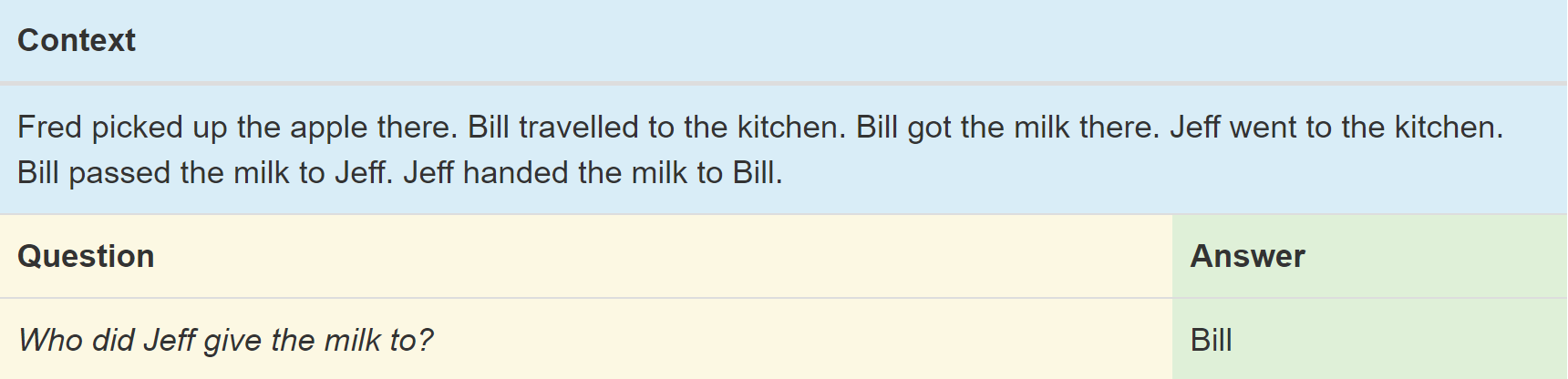
这项任务(#5)测试神经网络对三个对象之间存在关系的行为的理解。从语法上讲,它测试的是,网络是否可以区分主体,直接对象和间接对象。在这种情况下,问题在最后一句中问的是间接对象 - 从 Jeff 那里收到牛奶的人。因此,网络必须要区分出,第五句的主体是 Bill,Jeff 是宾语,以及第六句的主题是 Jeff。当然,我们的网络没有经过任何的主语或宾语识别的训练,所以必须从训练数据中的例子中推断出这种理解。
系统必须解决的另一个小问题是理解整个数据集中使用的各种同义词。 杰夫把牛奶 “ handed ” 给比尔,机器可能会比较容易理解 “ give ” 或 “ pass ” 这样的动词,但是 “ handed ” 这样的词则不一定容易理解。但是,在同义词这方面,神经网络的学习不必从头开始。因为词向量的表示形式会提供一些帮助,词向量可以存储有关单词的定义及其与其他单词关系的信息。相似词义的词具有相似的矢量,这意味着网络可以将它们看作几乎相同的单词。对于词向量,这里我们将使用斯坦福的 GloVe。
许多 QA 任务都有一个限制,就是强制上下文中包含用于答案的确切词汇。在我们的例子中,可以在上下文中找到答案 “ Bill ”。我们将利用这个限制来优化结果,因为我们可以在上下文中搜索最接近我们最终结果的词语。
Download Dataset
注意:我们可能需要几分钟才能下载并解压缩所有这些数据,在运行完接下来的三个代码片段后,我们将会下载完成 bAbI 和 GloVe,并将它们解压出来,以便在我们的网络中使用它们。
glove_zip_file = "glove.6B.zip"
glove_vectors_file = "glove.6B.50d.txt"

# 15 MB
data_set_zip = "tasks_1-20_v1-2.tar.gz"

#Select "task 5"
train_set_file = "qa5_three-arg-relations_train.txt"
test_set_file = "qa5_three-arg-relations_test.txt"

train_set_post_file = "tasks_1-20_v1-2/en/"+train_set_file
test_set_post_file = "tasks_1-20_v1-2/en/"+test_set_file
try:
from urllib.request import urlretrieve, urlopen
except ImportError:
from urllib import urlretrieve
from urllib2 import urlopen
#large file - 862 MB
if (not os.path.isfile(glove_zip_file) and
not os.path.isfile(glove_vectors_file)):
urlretrieve ("http://nlp.stanford.edu/data/glove.6B.zip",
glove_zip_file)
if (not os.path.isfile(data_set_zip) and
not (os.path.isfile(train_set_file) and os.path.isfile(test_set_file))):
urlretrieve ("https://s3.amazonaws.com/text-datasets/babi_tasks_1-20_v1-2.tar.gz",
data_set_zip)def unzip_single_file(zip_file_name, output_file_name):
"""
If the output file is already created, don't recreate
If the output file does not exist, create it from the zipFile
"""
if not os.path.isfile(output_file_name):
with open(output_file_name, 'wb') as out_file:
with zipfile.ZipFile(zip_file_name) as zipped:
for info in zipped.infolist():
if output_file_name in info.filename:
with zipped.open(info) as requested_file:
out_file.write(requested_file.read())
return
def targz_unzip_single_file(zip_file_name, output_file_name, interior_relative_path):
if not os.path.isfile(output_file_name):
with tarfile.open(zip_file_name) as un_zipped:
un_zipped.extract(interior_relative_path+output_file_name)
unzip_single_file(glove_zip_file, glove_vectors_file)
targz_unzip_single_file(data_set_zip, train_set_file, "tasks_1-20_v1-2/en/")
targz_unzip_single_file(data_set_zip, test_set_file, "tasks_1-20_v1-2/en/")Parsing GloVe and Handling Unknown Tokens
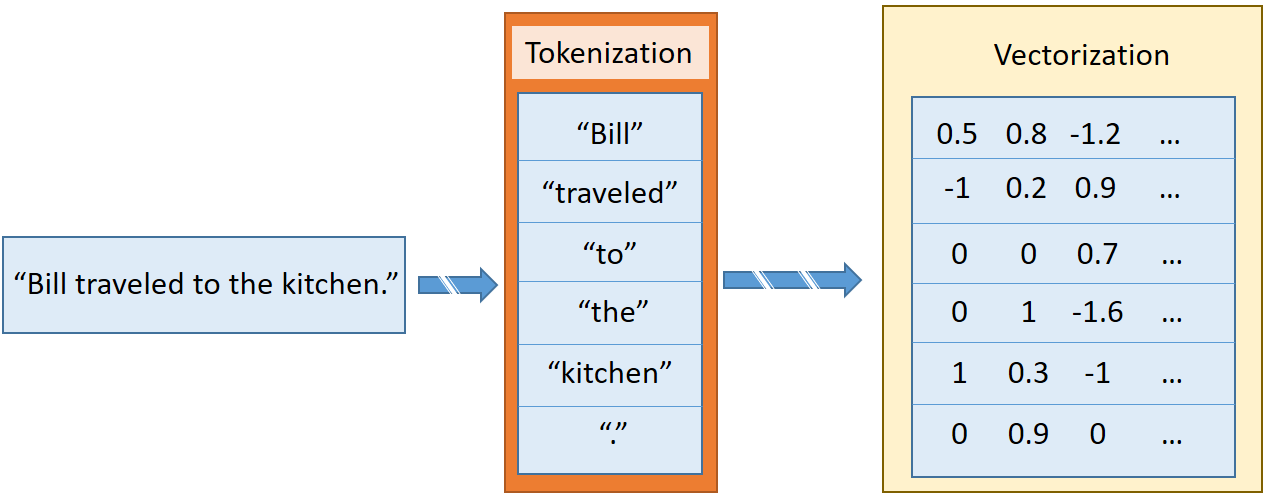
这里,我们会再讨论一个如何将 sentence 通过 GloVe 转换成 vector sequence 或者是 matrix 的方法。这个方法需要将字符串分解成一个一个的单词,标点符号等。例如:“ Bill traveled to the kitchen, ” 会被分解成为六个单词,前五个是英语单词,第六个是标点符号。我们会将每一个部分进行矢量化,如下图所示:
在 bAbI 中的某些任务中,我们将遇到一些不在 GloVe 中的单词。为了让神经网络能够处理这些未知的单词,我们需要给这些单词的一个特殊的矢量化方式。常见的做法是用一个单一的 UNK 矢量来替换所有未知单词。但这不一定是最好的方法,又是,我们可以随机的为每个唯一的未知单词安排一个词向量。
当我们第一次遇到一个新的未知单词时,我们只需从原始 Glove 矢量的(高斯近似)分布中绘制一个新的矢量,并将该矢量添加回 GloVe 单词图中。为了收集分布超参数,Numpy具有自动计算方差和均值的功能。
下面的 fill_unk 函数将会对未见过的单词生成一个新的单词矢量。
# Deserialize GloVe vectors
glove_wordmap = {}
with open(glove_vectors_file, "r", encoding="utf8") as glove:
    for line in glove:
        name, vector = tuple(line.split(" ", 1))
        glove_wordmap[name] = np.fromstring(vector, sep=" ")
wvecs = []
for item in glove_wordmap.items():
wvecs.append(item[1])
s = np.vstack(wvecs)
# Gather the distribution hyperparameters
v = np.var(s,0)
m = np.mean(s,0)
RS = np.random.RandomState()
def fill_unk(unk):
global glove_wordmap
glove_wordmap[unk] = RS.multivariate_normal(m,np.diag(v))
return glove_wordmap[unk]Known or Unknown
bAbI 任务的有限词汇量意味着即使不知道单词的含义,网络也可以学习单词之间的关系。然而,为了学习的速度,我们应该选择具有固有含义的矢量化。为此,我们对斯坦福大学 GLoVe 词汇矢量化数据集中存在的单词进行贪婪搜索(Greedy Search),如果单词不存在,那么我们用一个未知的随机创建的新表示填充整个单词。
通过这种定义,我们给出了下面的一个函数 sentence2sequence
def sentence2sequence(sentence):
    """
    Turns an input paragraph into an (m,d) matrix,
        where n is the number of tokens in the sentence
        and d is the number of dimensions each word vector has.

      TensorFlow doesn't need to be used here, as simply
      turning the sentence into a sequence based off our
      mapping does not need the computational power that
      TensorFlow provides. Normal Python suffices for this task.
    """
    tokens = sentence.strip('"(),-').lower().split(" ")
    rows = []
    words = []
    #Greedy search for tokens
    for token in tokens:
        i = len(token)
        while len(token) > 0:
            word = token[:i]
            if word in glove_wordmap:
                rows.append(glove_wordmap[word])
                words.append(word)
                token = token[i:]
                i = len(token)
                continue
            else:
                i = i-1
            if i == 0:
                # word OOV
                # https://arxiv.org/pdf/1611.01436.pdf
                rows.append(fill_unk(token))
                words.append(token)
                break
    return np.array(rows), words
现在我们可以将每个问题所需的所有数据打包在一起,包括上下文的矢量,问题和答案。在 bAbI 中,上下文由编号的句子序列定义,将上下文序列化为与一个上下文相关的句子列表。问题和答案位于同一行,由 \t 分隔,因此我们可以使用 \t 作为特定行是否引用问题的标记。当编号重置时,未来的问题将引用新的上下文(注意,通常有多个问题对应于单个上下文)。答案还包含我们保留但不需要使用的另一条信息:与参考顺序中回答问题所需的句子相对应的数字。在我们的系统中,网络会自学自己需要哪些句子来回答问题。
def contextualize(set_file):
    """
    Read in the dataset of questions and build question+answer -> context sets.
    Output is a list of data points, each of which is a 7-element tuple containing:
        The sentences in the context in vectorized form.
        The sentences in the context as a list of string tokens.
        The question in vectorized form.
        The question as a list of string tokens.
        The answer in vectorized form.
        The answer as a list of string tokens.
        A list of numbers for supporting statements, which is currently unused.
    """
    data = []
    context = []
    with open(set_file, "r", encoding="utf8") as train:
        for line in train:
            l, ine = tuple(line.split(" ", 1))
            # Split the line numbers from the sentences they refer to.
            if l is "1":
                # New contexts always start with 1,
                # so this is a signal to reset the context.
                context = []
            if "\t" in ine:
                # Tabs are the separator between questions and answers,
                # and are not present in context statements.
                question, answer, support = tuple(ine.split("\t"))
                data.append((tuple(zip(*context))+
                             sentence2sequence(question)+
                             sentence2sequence(answer)+
                             ([int(s) for s in support.split()],)))
                # Multiple questions may refer to the same context, so we don't reset it.
            else:
                # Context sentence.
                context.append(sentence2sequence(ine[:-1]))
    return data
train_data = contextualize(train_set_post_file)
test_data = contextualize(test_set_post_file)
final_train_data = []
def finalize(data):
"""
Prepares data generated by contextualize() for use in the network.
"""
final_data = []
for cqas in train_data:
contextvs, contextws, qvs, qws, avs, aws, spt = cqas
lengths = itertools.accumulate(len(cvec) for cvec in contextvs)
context_vec = np.concatenate(contextvs)
context_words = sum(contextws,[])
# Location markers for the beginnings of new sentences.
sentence_ends = np.array(list(lengths))
final_data.append((context_vec, sentence_ends, qvs, spt, context_words, cqas, avs, aws))
return np.array(final_data)
final_train_data = finalize(train_data)
final_test_data = finalize(test_data)Defining Hyperparameters
此时,我们已经准备好了我们的训练数据和测试数据。接下来的任务是构建用来理解数据的网络。我们首先重置 TensorFlow 的 default graph,这样我们就可以随时再次运行网络,如果我们想要改变某些东西的话。(TensorFlow 的初学者,应该经常踩过很多次变量名已经存在,不能再创建的坑吧。。)
tf.reset_default_graph()由于这是实际网络的开始,我们还要定义网络所需的所有常量。我们称之为“超参数”,因为它们定义了网络的结构和训练方式:
# Hyperparameters

# The number of dimensions used to store data passed between recurrent layers in the network.
recurrent_cell_size = 128

# The number of dimensions in our word vectorizations.
D = 50

# How quickly the network learns. Too high, and we may run into numeric instability
# or other issues.
learning_rate = 0.005

# Dropout probabilities. For a description of dropout and what these probabilities are,
# see Entailment with TensorFlow.
input_p, output_p = 0.5, 0.5

# How many questions we train on at a time.
batch_size = 128

# Number of passes in episodic memory. We'll get to this later.
passes = 4

# Feed Forward layer sizes: the number of dimensions used to store data passed from feed-forward layers.
ff_hidden_size = 256

weight_decay = 0.00000001
# The strength of our regularization. Increase to encourage sparsity in episodic memory,
# but makes training slower. Don't make this larger than leraning_rate.

training_iterations_count = 400000
# How many questions the network trains on each time it is trained.
# Some questions are counted multiple times.

display_step = 100
# How many iterations of training occur before each validation check.
Network Structure
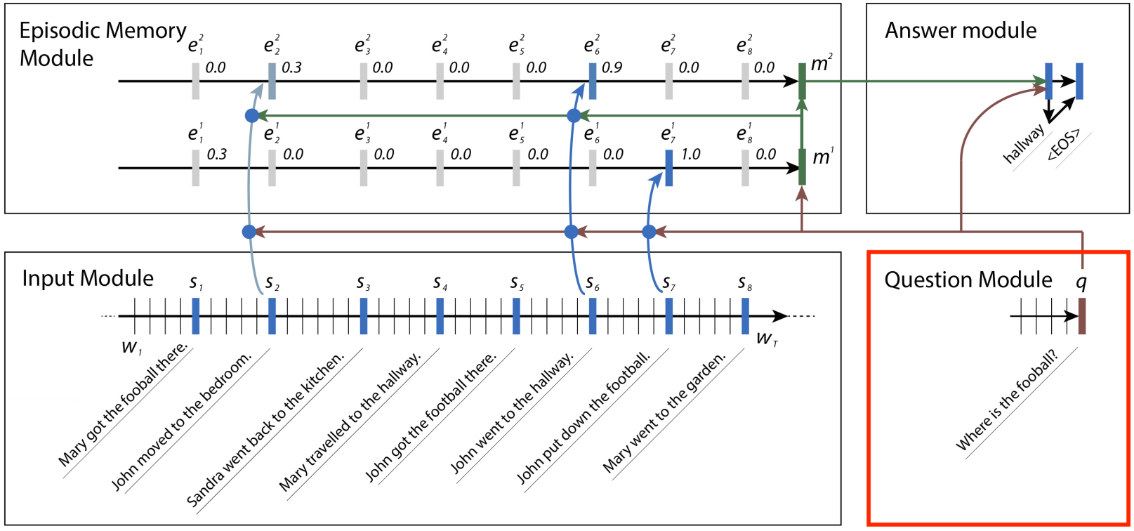
通过超参数,我们来描述网络结构。这个网络的结构被分成四个模块,在 “ Ask Me Anything:Dynamic Memory Networks for Natural Language Processing ” 论文中有描述。
首先来说一下这个网络的构建思路,它其实是根据人是如何做阅读理解,来创建的,那么,回忆一下大家是怎么做英语阅读理解的,是不是首先一句一句的读上下文的每一个句子,读完后,就会好像有点记住这句话讲的是啥,也就是说,每读完一句话,我们会创建一个记忆(memory),但是这个记忆也不是这个句子本身,我们记住的不是这个句子是怎么写的,哪个词会跟着哪个词,我们记住的是这句话讲的什么东西,讲的内容,在这个网络中被称为 fact。好了,读了句子,产生了关于 fact 的记忆,当我们在回答问题的时候,我们会读完题目后,在重新审视文本中找相关的内容,来试图回答问题,在这个网络中,会将问题与每个 fact 进行比较,最后找到答案。这就是这个网络的基本思路了。
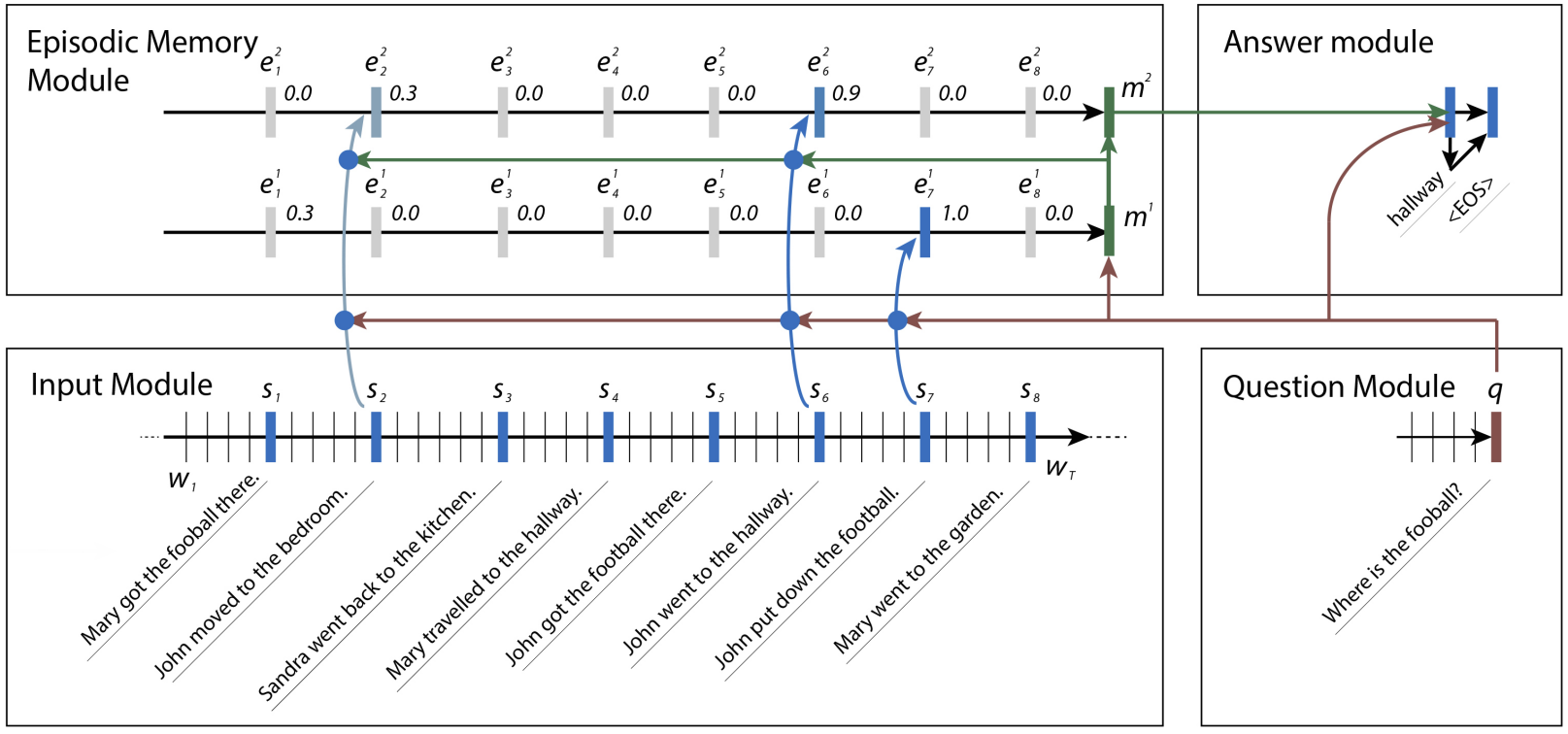
有时,一个事实会引导我们到另一个事实。例如上图的例子中,网络可能想要查找足球的位置。它可能会搜索有关足球的句子,发现约翰是最后一个接触足球的人,然后搜索关于约翰的句子,以发现约翰曾在卧室和走廊里。 一旦它意识到约翰已经走到了走廊的最后,它就可以回答这个问题并自信地说足球在走廊里。
网络内部的一共有四个模块一起合作来解决 bAbI 问题。接下来,我们来一个一个的分析网络中的每一个部分。
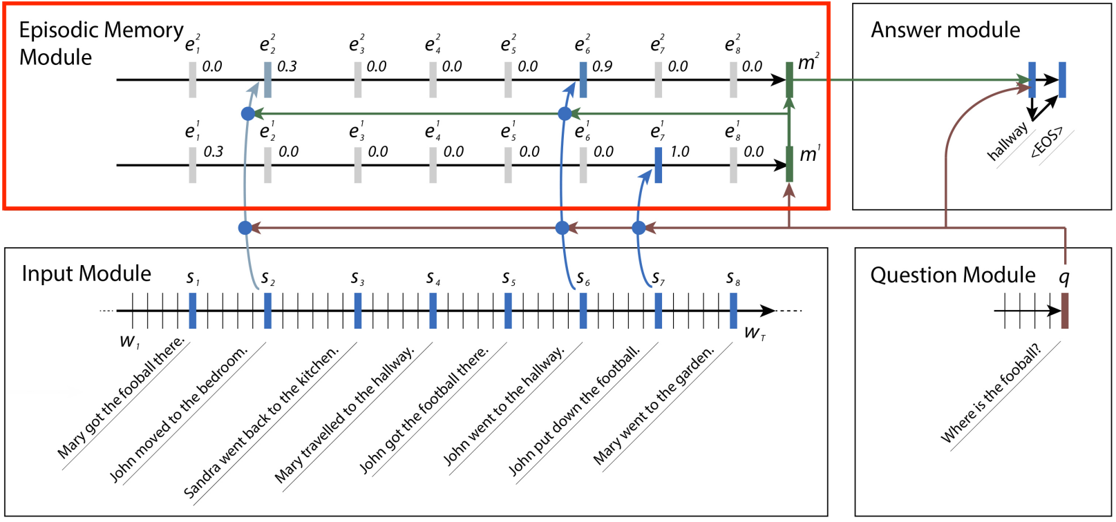
- 1. Input Module
输入模块是动态存储器网络用来提出答案的四个模块中的第一个模块,它包含一个简单的输入端和门控循环单元(GRU)(TensorFlow的tf.contrib.nn.GRUCell )用来收集证据(evidence)。每条证据 (evidence) 或事实 (fact) 是对应于上下文中的单个句子的,他们是 RNN 到这个步骤时的输出。这需要一些非 TensorFlow 预处理(词向量处理),以便在以后的模块中使用。我们会在稍后处理这些外部处理的过程。
我们可以使用 TensorFlow 的 gather_nd 处理的数据来选择相应的输出。函数 gather_nd 是一个非常有用的工具,我建议先看看 API文档 以了解其工作原理。
# Input Module

# Context: A [batch_size, maximum_context_length, word_vectorization_dimensions] tensor
# that contains all the context information.
context = tf.placeholder(tf.float32, [None, None, D], "context")
context_placeholder = context # I use context as a variable name later on

# input_sentence_endings: A [batch_size, maximum_sentence_count, 2] tensor that
# contains the locations of the ends of sentences.
input_sentence_endings = tf.placeholder(tf.int32, [None, None, 2], "sentence")

# recurrent_cell_size: the number of hidden units in recurrent layers.
input_gru = tf.contrib.rnn.GRUCell(recurrent_cell_size)

# input_p: The probability of maintaining a specific hidden input unit.
# Likewise, output_p is the probability of maintaining a specific hidden output unit.
gru_drop = tf.contrib.rnn.DropoutWrapper(input_gru, input_p, output_p)

# dynamic_rnn also returns the final internal state. We don't need that, and can
# ignore the corresponding output (_).
input_module_outputs, _ = tf.nn.dynamic_rnn(gru_drop, context, dtype=tf.float32, scope = "input_module")

# cs: the facts gathered from the context.
cs = tf.gather_nd(input_module_outputs, input_sentence_endings)
# to use every word as a fact, useful for tasks with one-sentence contexts
s = input_module_outputs- 2. Question Module
问题模块是第二个模块,可以说是最简单的。它仅仅由另一个GRU通过问题的文本。我们可以简单地传递最终状态,而不是一些证据(evidence),因为数据集中的所有的问题只有一个句子的长度。
# Question Module

# query: A [batch_size, maximum_question_length, word_vectorization_dimensions] tensor
#  that contains all of the questions.

query = tf.placeholder(tf.float32, [None, None, D], "query")

# input_query_lengths: A [batch_size, 2] tensor that contains question length information.
# input_query_lengths[:,1] has the actual lengths; input_query_lengths[:,0] is a simple range()
# so that it plays nice with gather_nd.
input_query_lengths = tf.placeholder(tf.int32, [None, 2], "query_lengths")

question_module_outputs, _ = tf.nn.dynamic_rnn(gru_drop, query, dtype=tf.float32,
                                               scope = tf.VariableScope(True, "input_module"))

# q: the question states. A [batch_size, recurrent_cell_size] tensor.
q = tf.gather_nd(question_module_outputs, input_query_lengths)- 3. Episodic Memory Module
我们的第三个模块,情景记忆模块(Episodic Memory Module),这是事情开始变得有趣的地方。它使用注意力来执行多次传递,每次传递由 GRU 组成,迭代输入。根据当时对相应事实的关注程度,每次传递中的每次迭代都会对当前内存进行加权更新。
Hard Attention VS Soft Attention
神经网络中的注意力最初是为图像分析而设计的,特别是对于图像某些部分比其他部分更与结果相关的情况。网络使用注意力机制,在执行任务时进行进一步分析需要额外注意的位置,例如查找图像中对象的位置,面部识等图像任务。
目前注意力机制的主要的问题是,或者说硬注意力机制(Hard-Attention)的问题,是不容易被优化。硬注意力机制的意思是,抽取仅仅某一个位置来额外关注。与大多数其他神经网络一样,我们的 Optimizer 是根据输入和权重计算损失函数的导数,由于其二元性质(回答正确或者是回答错误),硬性注意力根本不可区分。相反,我们不得不使用被称为 “ 软性关注 ”(Soft-Attention)的实值版本,该版本将所有可能使用的输入位置与使用某种形式的权重相结合。值得庆幸的是,权重是完全可以区分的,并且可以正常训练。 虽然可以硬注意力机制也可以用来学习,但是它的学习过程比软性注意要困难得多,有时表现得更差。因此,我们将选择使用 Soft Attention。而我们完全不用担心编码的问题,因为 TensorFlow 已经实现了。
在这个模型中,我们计算注意力的方法是利用相似度作为指标,相似度是由:每个事实(fact),当前的记忆(memory)还有问题(question)计算得来。我们将结果通过双层前馈网络传递给每个 fact 的注意力常量。然后,我们通过在输入上使用 GRU 进行加权传递来修改 memory(由相应的注意力常数加权)。为了避免当上下文短于矩阵的全部长度时将不正确的信息添加到 memory 中,我们创建了一个 mask 来保证最短的长度。
另一个值得注意的方面是关注 mask 几乎总是在 recurrent layer 使用。对于图像来说,这个 wrapping 最可能发生在卷积层(最可能是直接在映射到图像中的位置),对于自然语言而言,wrapping 最可能发生在 recurrent layer。
# Episodic Memory

# make sure the current memory (i.e. the question vector) is broadcasted along the facts dimension
size = tf.stack([tf.constant(1),tf.shape(cs)[1], tf.constant(1)])
re_q = tf.tile(tf.reshape(q,[-1,1,recurrent_cell_size]),size)


# Final output for attention, needs to be 1 in order to create a mask
output_size = 1

# Weights and biases
attend_init = tf.random_normal_initializer(stddev=0.1)
w_1 = tf.get_variable("attend_w1", [1,recurrent_cell_size*7, recurrent_cell_size],
                      tf.float32, initializer = attend_init)
w_2 = tf.get_variable("attend_w2", [1,recurrent_cell_size, output_size],
                      tf.float32, initializer = attend_init)

b_1 = tf.get_variable("attend_b1", [1, recurrent_cell_size],
                      tf.float32, initializer = attend_init)
b_2 = tf.get_variable("attend_b2", [1, output_size],
                      tf.float32, initializer = attend_init)

# Regulate all the weights and biases
tf.add_to_collection(tf.GraphKeys.REGULARIZATION_LOSSES, tf.nn.l2_loss(w_1))
tf.add_to_collection(tf.GraphKeys.REGULARIZATION_LOSSES, tf.nn.l2_loss(b_1))
tf.add_to_collection(tf.GraphKeys.REGULARIZATION_LOSSES, tf.nn.l2_loss(w_2))
tf.add_to_collection(tf.GraphKeys.REGULARIZATION_LOSSES, tf.nn.l2_loss(b_2))

def attention(c, mem, existing_facts):
    """
    Custom attention mechanism.
    c: A [batch_size, maximum_sentence_count, recurrent_cell_size] tensor
        that contains all the facts from the contexts.
    mem: A [batch_size, maximum_sentence_count, recurrent_cell_size] tensor that
        contains the current memory. It should be the same memory for all facts for accurate results.
    existing_facts: A [batch_size, maximum_sentence_count, 1] tensor that
        acts as a binary mask for which facts exist and which do not.

    """
    with tf.variable_scope("attending") as scope:
        # attending: The metrics by which we decide what to attend to.
        attending = tf.concat([c, mem, re_q, c * re_q,  c * mem, (c-re_q)**2, (c-mem)**2], 2)

        # m1: First layer of multiplied weights for the feed-forward network.
        #     We tile the weights in order to manually broadcast, since tf.matmul does not
        #     automatically broadcast batch matrix multiplication as of TensorFlow 1.2.
        m1 = tf.matmul(attending * existing_facts,
                       tf.tile(w_1, tf.stack([tf.shape(attending)[0],1,1]))) * existing_facts
        # bias_1: A masked version of the first feed-forward layer's bias
        #     over only existing facts.

        bias_1 = b_1 * existing_facts

        # tnhan: First nonlinearity. In the original paper, this is a tanh nonlinearity;
        #        choosing relu was a design choice intended to avoid issues with
        #        low gradient magnitude when the tanh returned values close to 1 or -1.
        tnhan = tf.nn.relu(m1 + bias_1)

        # m2: Second layer of multiplied weights for the feed-forward network.
        #     Still tiling weights for the same reason described in m1's comments.
        m2 = tf.matmul(tnhan, tf.tile(w_2, tf.stack([tf.shape(attending)[0],1,1])))

        # bias_2: A masked version of the second feed-forward layer's bias.
        bias_2 = b_2 * existing_facts

        # norm_m2: A normalized version of the second layer of weights, which is used
        #     to help make sure the softmax nonlinearity doesn't saturate.
        norm_m2 = tf.nn.l2_normalize(m2 + bias_2, -1)

        # softmaxable: A hack in order to use sparse_softmax on an otherwise dense tensor.
        #     We make norm_m2 a sparse tensor, then make it dense again after the operation.
        softmax_idx = tf.where(tf.not_equal(norm_m2, 0))[:,:-1]
        softmax_gather = tf.gather_nd(norm_m2[...,0], softmax_idx)
        softmax_shape = tf.shape(norm_m2, out_type=tf.int64)[:-1]
        softmaxable = tf.SparseTensor(softmax_idx, softmax_gather, softmax_shape)
        return tf.expand_dims(tf.sparse_tensor_to_dense(tf.sparse_softmax(softmaxable)),-1)

# facts_0s: a [batch_size, max_facts_length, 1] tensor
#     whose values are 1 if the corresponding fact exists and 0 if not.
facts_0s = tf.cast(tf.count_nonzero(input_sentence_endings[:,:,-1:],-1,keep_dims=True),tf.float32)


with tf.variable_scope("Episodes") as scope:
    attention_gru = tf.contrib.rnn.GRUCell(recurrent_cell_size)

    # memory: A list of all tensors that are the (current or past) memory state
    #   of the attention mechanism.
    memory = [q]

    # attends: A list of all tensors that represent what the network attends to.
    attends = []
    for a in range(passes):
        # attention mask
        attend_to = attention(cs, tf.tile(tf.reshape(memory[-1],[-1,1,recurrent_cell_size]),size),
                              facts_0s)

        # Inverse attention mask, for what's retained in the state.
        retain = 1-attend_to

        # GRU pass over the facts, according to the attention mask.
        while_valid_index = (lambda state, index: index < tf.shape(cs)[1])
        update_state = (lambda state, index: (attend_to[:,index,:] *
                                                 attention_gru(cs[:,index,:], state)[0] +
                                                 retain[:,index,:] * state))
        # start loop with most recent memory and at the first index
        memory.append(tuple(tf.while_loop(while_valid_index,
                          (lambda state, index: (update_state(state,index),index+1)),
                           loop_vars = [memory[-1], 0]))[0])

        attends.append(attend_to)

        # Reuse variables so the GRU pass uses the same variables every pass.
scope.reuse_variables()- 4. Answer Module
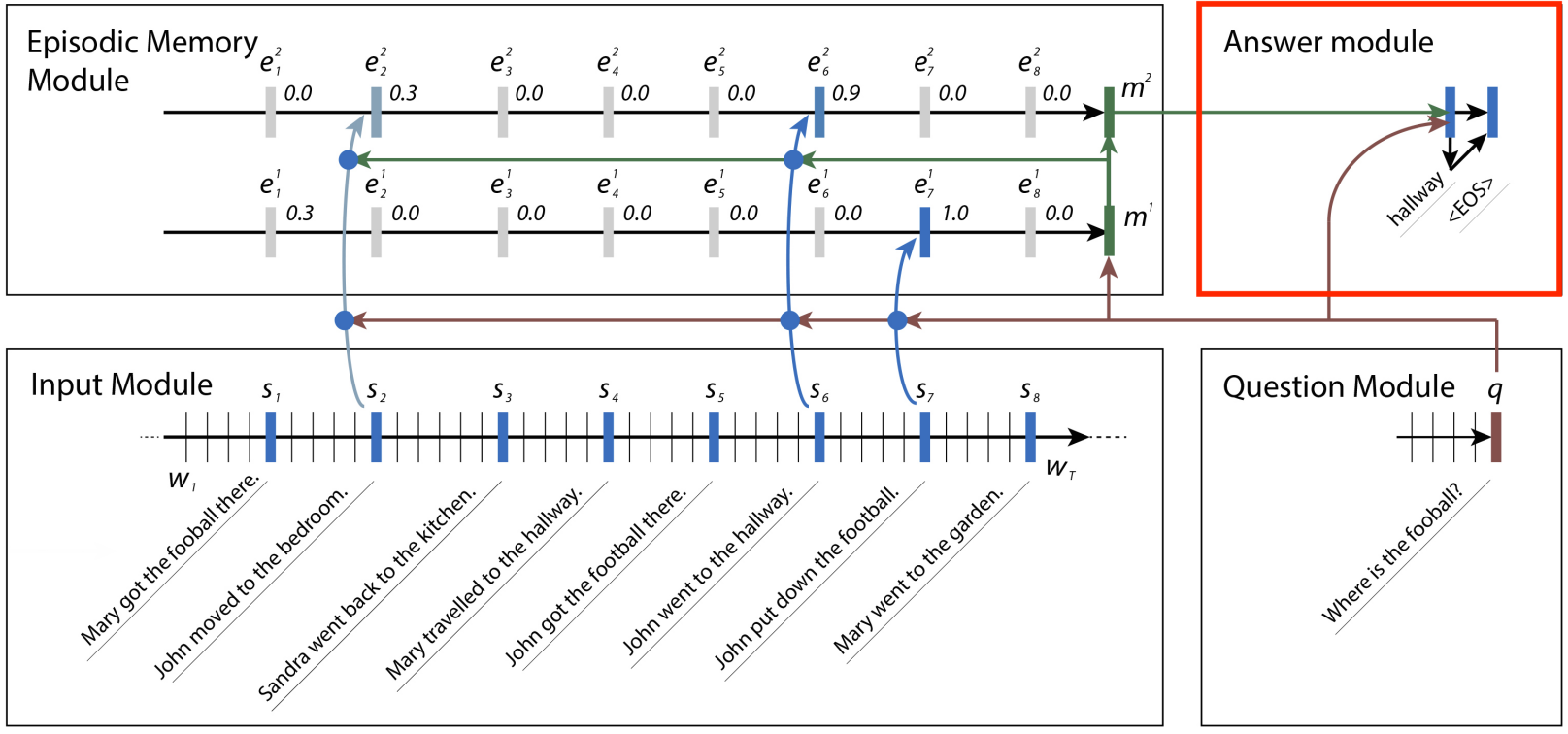
最后一个模块是答案模块,它从问题和情节记忆模块的输出中使用完全连接层指向最后的“最终结果”单词向量,并且距离结果,找到最近的单词最为最终结果输出。
# Answer Module

# a0: Final memory state. (Input to answer module)
a0 = tf.concat([memory[-1], q], -1)

# fc_init: Initializer for the final fully connected layer's weights.
fc_init = tf.random_normal_initializer(stddev=0.1)

with tf.variable_scope("answer"):
    # w_answer: The final fully connected layer's weights.
    w_answer = tf.get_variable("weight", [recurrent_cell_size*2, D],
                               tf.float32, initializer = fc_init)
    # Regulate the fully connected layer's weights
    tf.add_to_collection(tf.GraphKeys.REGULARIZATION_LOSSES,
                     tf.nn.l2_loss(w_answer))

    # The regressed word. This isn't an actual word yet;
    #    we still have to find the closest match.
    logit = tf.expand_dims(tf.matmul(a0, w_answer),1)

    # Make a mask over which words exist.
    with tf.variable_scope("ending"):
        all_ends = tf.reshape(input_sentence_endings, [-1,2])
        range_ends = tf.range(tf.shape(all_ends)[0])
        ends_indices = tf.stack([all_ends[:,0],range_ends], axis=1)
        ind = tf.reduce_max(tf.scatter_nd(ends_indices, all_ends[:,1],
                                          [tf.shape(q)[0], tf.shape(all_ends)[0]]),
                            axis=-1)
        range_ind = tf.range(tf.shape(ind)[0])
        mask_ends = tf.cast(tf.scatter_nd(tf.stack([ind, range_ind], axis=1),
                                          tf.ones_like(range_ind), [tf.reduce_max(ind)+1,
                                                                    tf.shape(ind)[0]]), bool)
        # A bit of a trick. With the locations of the ends of the mask (the last periods in
        #  each of the contexts) as 1 and the rest as 0, we can scan with exclusive or
        #  (starting from all 1). For each context in the batch, this will result in 1s
        #  up until the marker (the location of that last period) and 0s afterwards.
        mask = tf.scan(tf.logical_xor,mask_ends, tf.ones_like(range_ind, dtype=bool))

    # We score each possible word inversely with their Euclidean distance to the regressed word.
    #  The highest score (lowest distance) will correspond to the selected word.
    logits = -tf.reduce_sum(tf.square(context*tf.transpose(tf.expand_dims(
                    tf.cast(mask, tf.float32),-1),[1,0,2]) - logit), axis=-1)
Optimizing Optimization
这里我们将采用 AdamOptimizer 来作为优化器,关于梯度下降优化器的选择,可以参考我的另一篇博客。
# Training

# gold_standard: The real answers.
gold_standard = tf.placeholder(tf.float32, [None, 1, D], "answer")
with tf.variable_scope('accuracy'):
    eq = tf.equal(context, gold_standard)
    corrbool = tf.reduce_all(eq,-1)
    logloc = tf.reduce_max(logits, -1, keep_dims = True)
    # locs: A boolean tensor that indicates where the score
    #  matches the minimum score. This happens on multiple dimensions,
    #  so in the off chance there's one or two indexes that match
    #  we make sure it matches in all indexes.
    locs = tf.equal(logits, logloc)

    # correctsbool: A boolean tensor that indicates for which
    #   words in the context the score always matches the minimum score.
    correctsbool = tf.reduce_any(tf.logical_and(locs, corrbool), -1)
    # corrects: A tensor that is simply correctsbool cast to floats.
    corrects = tf.where(correctsbool, tf.ones_like(correctsbool, dtype=tf.float32),
                        tf.zeros_like(correctsbool,dtype=tf.float32))

    # corr: corrects, but for the right answer instead of our selected answer.
    corr = tf.where(corrbool, tf.ones_like(corrbool, dtype=tf.float32),
                        tf.zeros_like(corrbool,dtype=tf.float32))
with tf.variable_scope("loss"):
    # Use sigmoid cross entropy as the base loss,
    #  with our distances as the relative probabilities. There are
    #  multiple correct labels, for each location of the answer word within the context.
    loss = tf.nn.sigmoid_cross_entropy_with_logits(logits = tf.nn.l2_normalize(logits,-1),
                                                   labels = corr)

    # Add regularization losses, weighted by weight_decay.
    total_loss = tf.reduce_mean(loss) + weight_decay * tf.add_n(
        tf.get_collection(tf.GraphKeys.REGULARIZATION_LOSSES))

# TensorFlow's default implementation of the Adam optimizer works. We can adjust more than
#  just the learning rate, but it's not necessary to find a very good optimum.
optimizer = tf.train.AdamOptimizer(learning_rate)

# Once we have an optimizer, we ask it to minimize the loss
#   in order to work towards the proper training.
opt_op = optimizer.minimize(total_loss)
# Initialize variables
init = tf.global_variables_initializer()
# Launch the TensorFlow session
sess = tf.Session()
sess.run(init)Train Network
当一切准备就绪,我们可以开始批量训练网络了!在训练的同时,我们应该检查网络在准确性方面的表现。可以使用验证集来完成此操作,该验证集取自测试数据,因此与训练数据没有重叠。
使用基于测试数据的验证集可以让我们更好地了解网络如何将其所学知识普遍化并将其应用于其他环境的能力。如果我们对训练数据进行验证,网络可能会过度训练 - 换句话说,学习具体的例子并记住答案,这对网络回答新问题并无帮助。
TQDM 可以帮助记录当前训练的进度。
def prep_batch(batch_data, more_data = False):
    """
        Prepare all the preproccessing that needs to be done on a batch-by-batch basis.
    """
    context_vec, sentence_ends, questionvs, spt, context_words, cqas, answervs, _ = zip(*batch_data)
    ends = list(sentence_ends)
    maxend = max(map(len, ends))
    aends = np.zeros((len(ends), maxend))
    for index, i in enumerate(ends):
        for indexj, x in enumerate(i):
            aends[index, indexj] = x-1
    new_ends = np.zeros(aends.shape+(2,))

    for index, x in np.ndenumerate(aends):
        new_ends[index+(0,)] = index[0]
        new_ends[index+(1,)] = x

    contexts = list(context_vec)
    max_context_length = max([len(x) for x in contexts])
    contextsize = list(np.array(contexts[0]).shape)
    contextsize[0] = max_context_length
    final_contexts = np.zeros([len(contexts)]+contextsize)

    contexts = [np.array(x) for x in contexts]
    for i, context in enumerate(contexts):
        final_contexts[i,0:len(context),:] = context
    max_query_length = max(len(x) for x in questionvs)
    querysize = list(np.array(questionvs[0]).shape)
    querysize[:1] = [len(questionvs),max_query_length]
    queries = np.zeros(querysize)
    querylengths = np.array(list(zip(range(len(questionvs)),[len(q)-1 for q in questionvs])))
    questions = [np.array(q) for q in questionvs]
    for i, question in enumerate(questions):
        queries[i,0:len(question),:] = question
    data = {context_placeholder: final_contexts, input_sentence_endings: new_ends,
                            query:queries, input_query_lengths:querylengths, gold_standard: answervs}
    return (data, context_words, cqas) if more_data else data
# Use TQDM if installed
tqdm_installed = False
try:
from tqdm import tqdm
tqdm_installed = True
except:
pass
# Prepare validation set
batch = np.random.randint(final_test_data.shape[0], size=batch_size*10)
batch_data = final_test_data[batch]
validation_set, val_context_words, val_cqas = prep_batch(batch_data, True)
# training_iterations_count: The number of data pieces to train on in total
# batch_size: The number of data pieces per batch
def train(iterations, batch_size):
training_iterations = range(0,iterations,batch_size)
if tqdm_installed:
# Add a progress bar if TQDM is installed
training_iterations = tqdm(training_iterations)
wordz = []
for j in training_iterations:
batch = np.random.randint(final_train_data.shape[0], size=batch_size)
batch_data = final_train_data[batch]
sess.run([opt_op], feed_dict=prep_batch(batch_data))
if (j/batch_size) % display_step == 0:
# Calculate batch accuracy
acc, ccs, tmp_loss, log, con, cor, loc = sess.run([corrects, cs, total_loss, logit,
context_placeholder,corr, locs],
feed_dict=validation_set)
# Display results
print("Iter " + str(j/batch_size) + ", Minibatch Loss= ",tmp_loss,
"Accuracy= ", np.mean(acc))
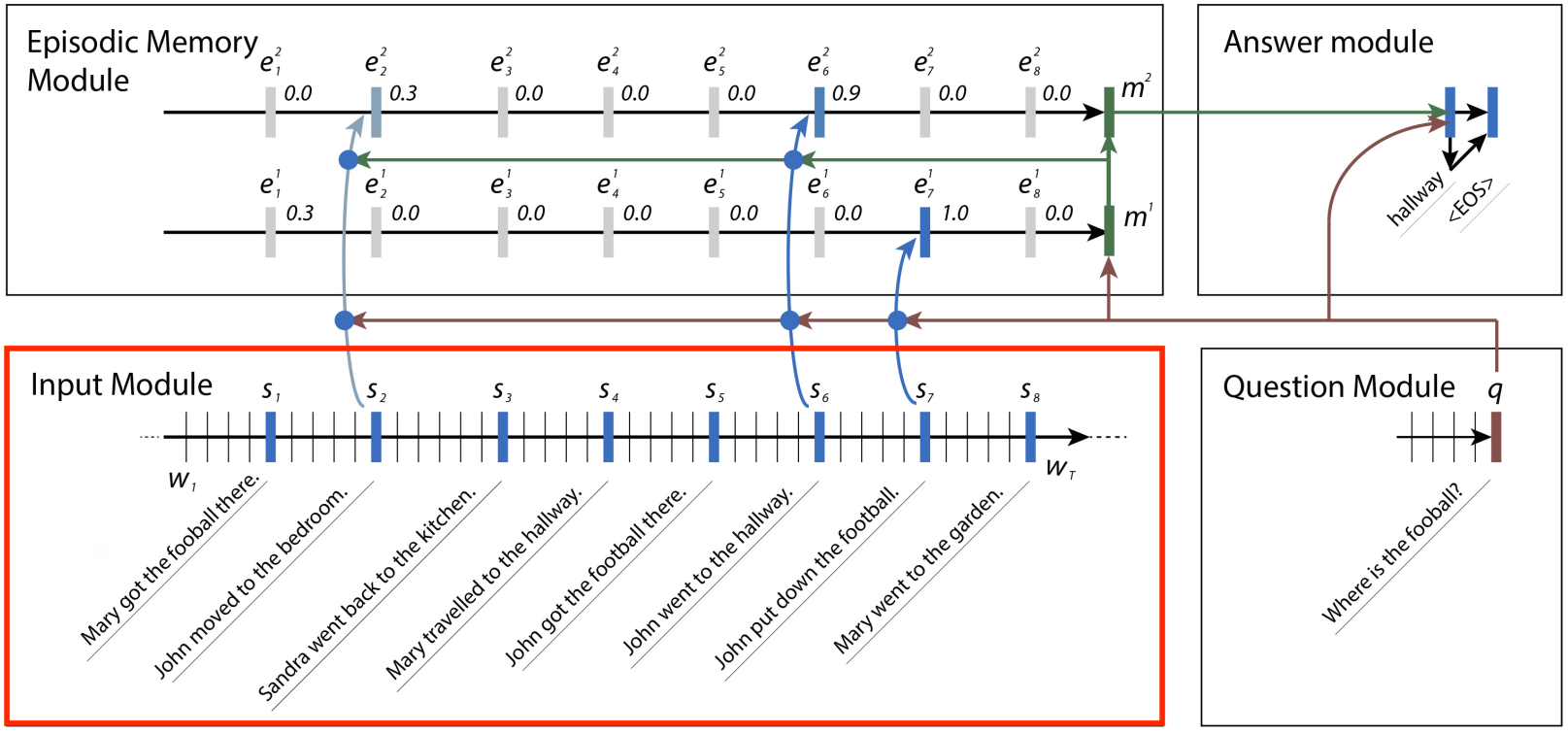
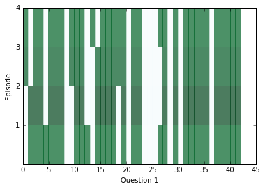
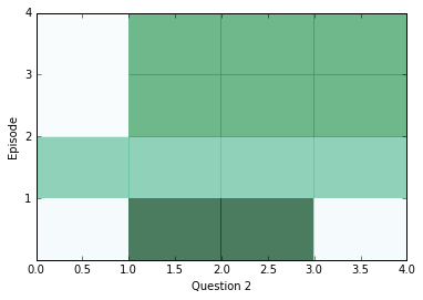
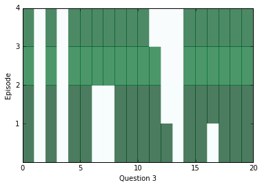
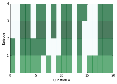
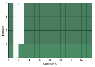
train(30000,batch_size) # Small amount of training for preliminary results在经过一段时间的训练后,让我们来看看从网络中得到了什么样的答案。在下面的图表中,我们可以看到关于我们上下文中所有句子的每一个段落的注意力分布情况; 较暗的颜色代表该集中对该句子的更多关注。
至少在每个问题的 episode 之间,我们可以看到了注意力的变化,但是有时候注意力能够在一个问题中找到答案,有时它会占用所有四个 episode。如果注意力似乎是空白的,它可能会饱和,这意味着它在关注所有事情,那么注意力机制就没有起到任何效果了。在这种情况下,你可以尝试用更高的weight_decay进行训练,以防止发生这种情况。在训练的后期,这种情况将会变得非常普遍。
为了看到上述问题的答案是什么,我们可以在上下文中使用我们的距离分数的位置作为索引,并查看该索引处的单词。
# Locations of responses within contexts
indices = np.argmax(n,axis=1)

# Locations of actual answers within contexts
indicesc = np.argmax(a,axis=1)

for i,e,cw, cqa in list(zip(indices, indicesc, val_context_words, val_cqas))[:limit]:
    ccc = " ".join(cw)
    print("TEXT: ",ccc)
    print ("QUESTION: ", " ".join(cqa[3]))
    print ("RESPONSE: ", cw[i], ["Correct", "Incorrect"][i!=e])
    print("EXPECTED: ", cw[e])
    print()
TEXT: mary travelled to the bedroom . mary journeyed to the bathroom . mary got the football there . mary passed the football to fred .
QUESTION: who received the football ?
RESPONSE: mary Incorrect
EXPECTED: fred
TEXT: bill grabbed the apple there . bill got the football there . jeff journeyed to the bathroom . bill handed the apple to jeff . jeff handed the apple to bill . bill handed the apple to jeff . jeff handed the apple to bill . bill handed the apple to jeff .
QUESTION: what did bill give to jeff ?
RESPONSE: apple Correct
EXPECTED: apple
TEXT: bill moved to the bathroom . mary went to the garden . mary picked up the apple there . bill moved to the kitchen . mary left the apple there . jeff got the football there . jeff went back to the kitchen . jeff gave the football to fred .
QUESTION: what did jeff give to fred ?
RESPONSE: apple Incorrect
EXPECTED: football
TEXT: jeff travelled to the bathroom . bill journeyed to the bedroom . jeff journeyed to the hallway . bill took the milk there . bill discarded the milk . mary moved to the bedroom . jeff went back to the bedroom . fred got the football there . bill grabbed the milk there . bill passed the milk to mary . mary gave the milk to bill . bill discarded the milk there . bill went to the kitchen . bill got the apple there .
QUESTION: who gave the milk to bill ?
RESPONSE: jeff Incorrect
EXPECTED: mary
TEXT: fred travelled to the bathroom . jeff went to the bathroom . mary went back to the bathroom . fred went back to the bedroom . fred moved to the office . mary went back to the bedroom . jeff got the milk there . bill journeyed to the garden . mary went back to the kitchen . fred went to the bedroom . mary journeyed to the bedroom . jeff put down the milk there . jeff picked up the milk there . bill went back to the office . mary went to the kitchen . jeff went back to the kitchen . jeff passed the milk to mary . mary gave the milk to jeff . jeff gave the milk to mary . mary got the football there . bill travelled to the bathroom . fred moved to the garden . fred got the apple there . mary handed the football to jeff . fred put down the apple . jeff left the football .
QUESTION: who received the football ?
RESPONSE: mary Incorrect
EXPECTED: jeff现在可以继续训练!为了获得良好的效果,可能需要长时间去训练,但最终应该能够达到非常高的精度(超过90%)。Jupyter Notebook的经验丰富的用户应该知道,只要保持相同的tf.Session,就可以随时中断训练并仍然保存网络所取得的进展,这很有用。
train(training_iterations_count, batch_size)# Final testing accuracy
print(np.mean(sess.run([corrects], feed_dict= prep_batch(final_test_data))[0]))至此,训练完成,我们应该可以得到 95% 的准确率。